


Design hyetographs is the free GeoStru geoapp that builds design hyetographs from the intensity-duration-frequency curve h = a·tⁿ, compares scenarios (return period, duration, shape), exports the time series for SWMM, HEC-HMS and Excel and produces the report as a PDF. It is the starting point of every hydrological-hydraulic design: sewers and drainage networks, hydraulic invariance, detention basins, culverts and channels, rainfall-runoff models. It runs in the browser, with no installation, also on the phone, and no data leaves your computer.
What a hyetograph is
A hyetograph is the chart that tells how much rain falls and when during a storm: time on the horizontal axis, intensity (mm/h) or rainfall depth (mm) of each interval on the vertical one. A design hyetograph is not an observed storm but a “synthetic” one built from the rainfall statistics of the site, the depth-duration-frequency curve h = a·tⁿ, which for a given return period (say 50 years) tells how much rain can fall in 10 minutes, in one hour, in one day. Once the storm duration and the time step are chosen, that depth is distributed in time with a shape: all equal (constant), with a peak (Chicago, alternating blocks), triangular. It is the input of hydrological and hydraulic models: from it you compute the flows reaching a sewer, a channel or a basin. Changing shape, duration or step changes the peak flow, which is why the application lets you compare several scenarios.
What it does
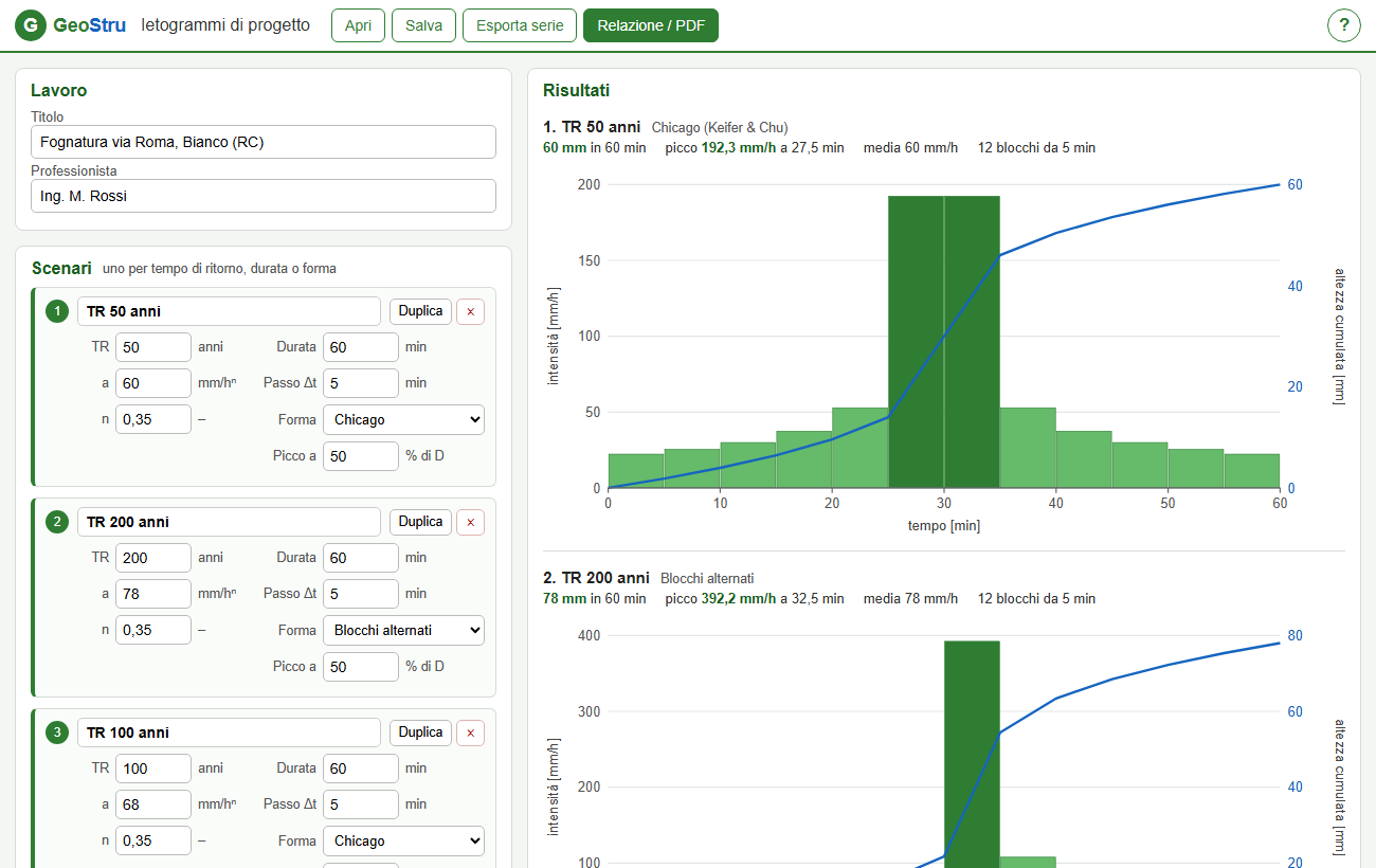
- Scenarios (up to 8): for each one the return period, the parameters a and n of the depth-duration curve (t in hours, h in mm), the duration D and the time step Δt in minutes, the hyetograph shape and the peak position. Everything is recomputed at every keystroke; Duplicate gives you the variant for another return period in a second.
- Four shapes: constant (equal blocks), Chicago (Keifer & Chu, 1957: every window centred on the peak has the depth given by the curve), triangular, alternating blocks. In all of them the total depth is a·(D/60)ⁿ, the one of the curve.
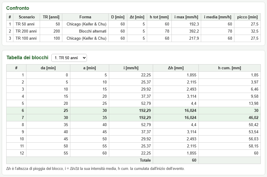
- Results: chart with intensity bars (mm/h) and cumulative depth (mm), total depth, peak intensity and peak time, mean intensity, number of blocks; comparison table between scenarios; block table (from, to, i, Δh, cumulative h) with the peak row highlighted.
- Export series: CSV for Excel (semicolon, decimal comma) or text for SWMM / HEC-HMS (tab, decimal point, minutes and mm/h), with the file name of your choice.
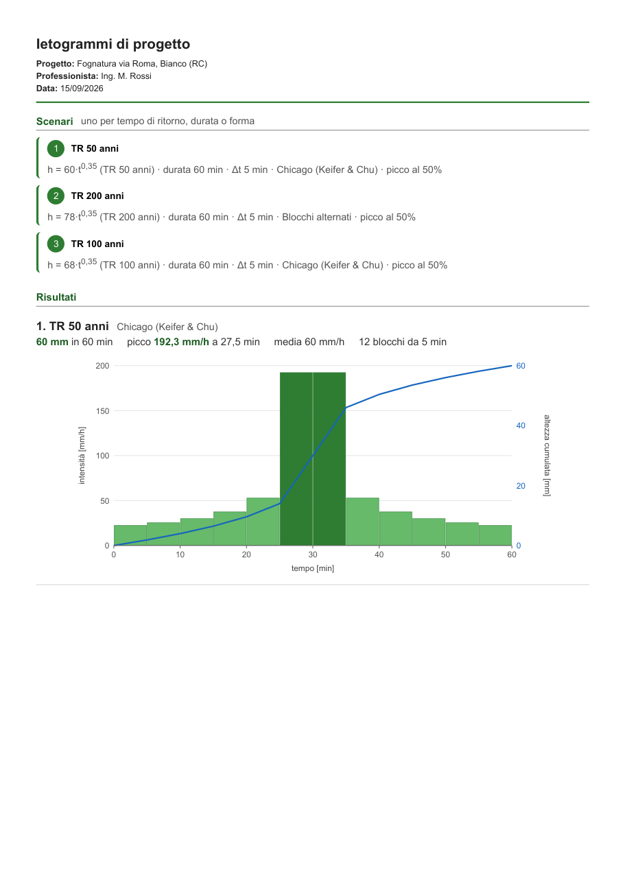
- Report / PDF: header with project title, professional and date, a summary line for each scenario, vector charts, comparison, block table and a Method paragraph with the formulas. Print it or save it as PDF from the browser.
- Estimate a and n from data: if you have the maximum depths per duration (1, 3, 6, 12, 24 hours…) and not the parameters, the least-squares line on ln h = ln a + n·ln t gives them with R² and residuals; one button puts them into a scenario.
- Save / Open: the work is saved to a
.jsonfile and reopened; it also stays in the browser between sessions, and the professional’s name is remembered.
How to use it
- Type the title and the professional (they go into the report).
- In each scenario enter a and n for the return period you need: these are the parameters published by hydrological yearbooks, basin plans and regional authorities (often already per return period). Mind the unit: here t is in hours; if your curve has t in minutes, convert a (ahours = amin·60ⁿ).
- Choose duration, time step and shape. For sewer networks the typical duration is the time of concentration or slightly more; a 5-minute step is what SWMM and HEC-HMS expect.
- Compare the scenarios in the table, export the series for the model, print the report.
From the hyetograph to hydraulic invariance
Hydraulic invariance (Italian regional regulations such as Lombardy R.R. 7/2019 and the similar rules of Veneto, Emilia-Romagna, Piedmont, Marche…) requires that after a land transformation the discharge released to the receiving body does not exceed the previous one: the difference must be stored in a basin or tank sized for a design storm with a prescribed return period (usually 50 years). The hyetograph is exactly that design storm: the Hydraulic invariance geoapp starts from the same data (curve h = a·tⁿ, return period, duration, Chicago / uniform / triangular shape, peak position), turns rainfall into discharge with the runoff coefficient and the time-of-concentration or Nash method, and computes the detention volume with the rainfall-only, the direct or the time-of-concentration method. Design hyetographs comes before and alongside: to understand and document the storm being used, to compare durations and shapes (the critical duration is the one giving the largest volume, and the shape changes the peak), to export the series and check the network or the basin with SWMM or HEC-HMS, and to estimate a and n when only observed depths are available. The same a and n then go into the Rainfall probability curves tab of the invariance app.
The report
With Report / PDF the page becomes the document: header, scenarios, charts, comparison, block table and the Method paragraph with the formulas used, ready to be attached to the project.
On the phone
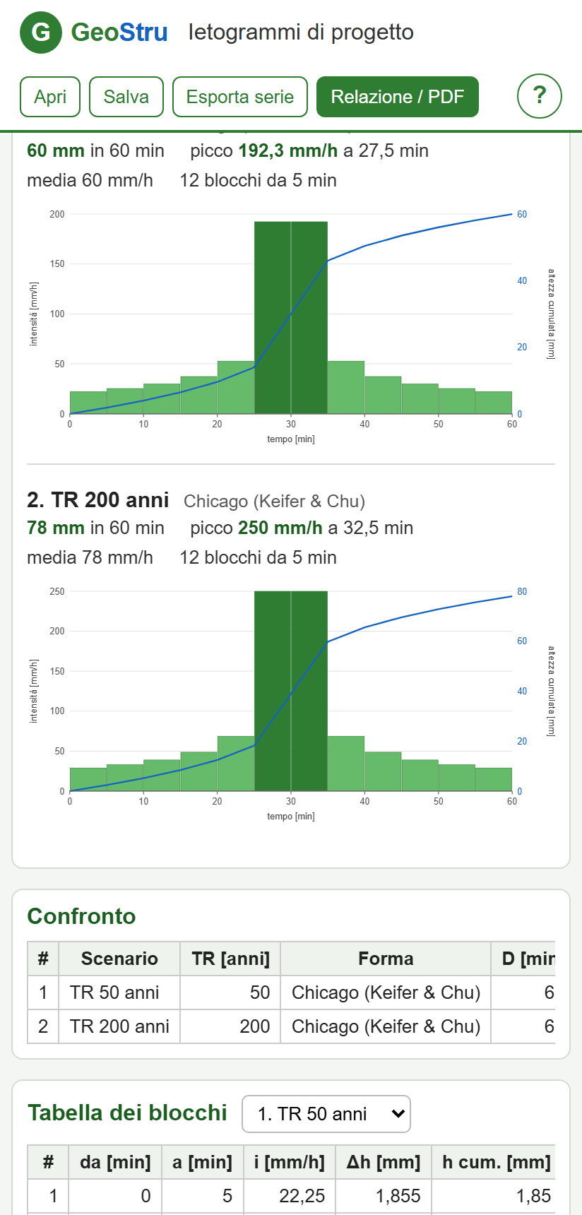
The page adapts to small screens: scenario fields go on one column and charts take the full width. Handy for a quick check in a meeting or on site.
Method
Rainfall depths come from the depth-duration curve h = a·tⁿ (t in hours). The duration D is split into N blocks of step Δt and the total depth is a·(D/60)ⁿ. Constant: equal blocks. Chicago (Keifer & Chu, 1957): for any window centred on the peak, with the fraction r before the peak, the depth equals the one of the curve; the cumulative depth before the peak at distance τ is a·r·(τ/r)ⁿ, after it a·(1−r)·(τ/(1−r))ⁿ. Triangular: intensity rising linearly to the peak at r·D and falling to zero, with area equal to the total depth. Alternating blocks: the increments a·[(kΔt)ⁿ − ((k−1)Δt)ⁿ] sorted from the largest, the first on the peak and the others alternately to the right and to the left. The instantaneous intensity at the Chicago peak is infinite: the blocks make it finite, and it depends on the chosen step. The estimate of a and n is the linear regression of ln h on ln t.
Related applications
Hydraulic invariance · Time of concentration · Uniform flow · Ditch hydraulic design · Soakaway wells
References
GeoStru Design hyetographs — version 1.0.5, 15 September 2026. Keifer C.J., Chu H.H. (1957), Synthetic storm pattern for drainage design, Journal of the Hydraulics Division, ASCE. Free application; the computation runs in the browser and no data is sent to the server. The interface is in Italian.
Apri