


Slug test – Hvorslev 1951 is the application for calculating the permeability of an aquifer, through the interpretation of data according to the Hvorslev model (1951).
The application allows saving and reopening projects, as well as generating a detailed calculation report with theoretical background. The interpretation graph of the in-situ measurements is also shown.
Do you have any suggestions for us? Do you have any questions or other requests? Contact us on +39 06 90289085, email: info@geostru.eu or WhatsApp +40 0737 283 854.
Slug tests
The slug test has become one of the most widely used methods for a quick estimation of the main hydrogeological parameters of aquifers, primarily the hydraulic conductivity. In particular, the speed and ease of execution of these hydrodynamic tests become of primary importance to meet the needs of modern methods for evaluating aquifer vulnerability and pollution risk.
A slug test consists of causing an instantaneous change in the piezometric level in a borehole of “not large” diameter (e.g., in a piezometer) and measuring the time required for the subsequent restoration of the initial conditions; this can be achieved in various ways, but the operationally simplest consists of introducing (or extracting) a known volume of water, or a solid of cylindrical shape, into the test hole.
For a given volume of solid “slug” used for the test, the rate of recovery of the original level will be directly related to the hydraulic conductivity of the tested aquifer.
The test can be carried out both as a falling head or a rising head, i.e., first inserting and then, once the original water level has been restored, extracting the volume from the test piezometer, which caused the unbalance of the original level.
The success of the test is tied to the carefulness of the operational choices regarding the correct data acquisition technique and achieving a significant variation of the water level in the piezometer; the latter will depend on the volume of the solid slug, the diameter of the borehole, and the permeability of the aquifer subjected to the test.
The advantages of using slug tests are numerous: they affect the entire screened length and, therefore, involve levels with different permeability of the same aquifer, providing different values of K, by virtue of the more or less marked inhomogeneity and anisotropy of the aquifer as a whole; therefore both the hydraulic conductivity of aquifers and aquitards can be determined; measurements of hydraulic conductivity are made in situ and this avoids errors that occur in laboratory tests performed on remolded soil samples; it is not necessary to extract water from the aquifer and this is particularly important in the case of contaminated groundwater; the tests are quick and low-cost, because pumping and observation wells are not necessary.
The use of the slug test, however, has limitations: only the hydraulic conductivity of the aquifer in the vicinity of the piezometer can be evaluated, which may not be representative of a very large area; hence the need to have an adequate number of test points for the extent of the area to be studied; in general, the storage coefficient S cannot be determined (Robert P. Chapuis, D.Chenaf, 2002).
Hvorslev Method (1951)
Following the classic Hvorslev method, reference is made to the undisturbed piezometric level, i.e., the static level; after the introduction (falling head test) and after the extraction of the solid slug (rising head test), the maximum head difference, measured immediately before the start of the relative recoveries, will be indicated as H0, while the dynamic recovery levels will be indicated as H1, H2,… Hn. When water is removed the test is called a bail test, when it is introduced a slug test.
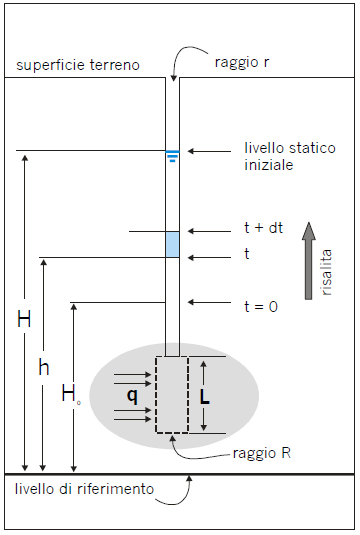
Figure 1 – Schematic representation of water rise
Referring to Figure 1, and assuming that water has been removed from the well, the inflow rate through the screen is:
![]()
from which the more general formula:
![]()
with F being a shape factor depending on the length and diameter of the screened part.
If q = q0 for t = 0, then q(t) asymptotically decreases towards zero as time passes.
Time lag Method
Hvorslev defined the basic time T0 (time lag) as:
![]()
Substituting the value into the previous expression, for h = H0 at time t = 0, we obtain:
![]()
By plotting time on the abscissa and the rise (on a logarithmic scale) on the ordinate, a linear trend is obtained. For values of (H – h) / (H – H0) = 0.37, then ln[(H – h) / (H – H0)] = -1, hence T0 = t, which is the definition of the time lag. To obtain K, the graph in Figure 2 is constructed, deriving T0 = 0.37.
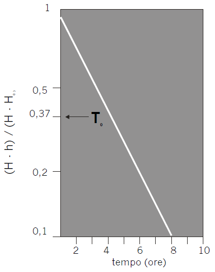
Figure 2 – Semi-logarithmic representation of the tests
Calculation of the shape factor
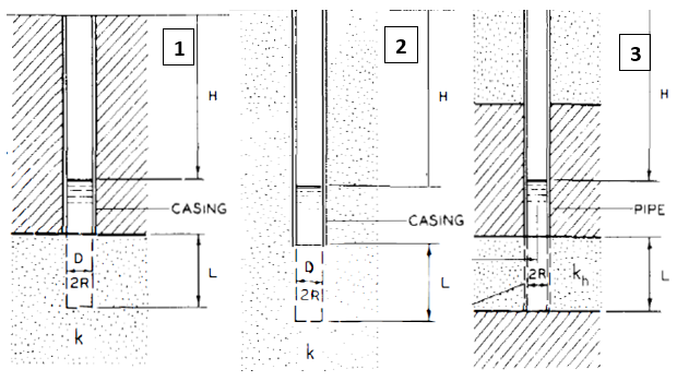
Figure 3 – Types of filter positions
Depending on the type of filter position (Figure 3), it is possible to derive the shape factor F.

Where:
- D = dfilter diameter (dw);
- L = wetted filter length (Lwetted);
- R = filter radius
Calculation of permeability K
Once the shape factor F is calculated, it is possible to derive K:

Where:
-
r = borehole radius